How to Concatenate in Google Sheets (Combine Cells without Losing Data)
Learn how to use CONCATENATE to combine cells in Google Sheets without losing data.
![[Featured image] Students learn how to concatenate in Google Sheets.](https://d3njjcbhbojbot.cloudfront.net/api/utilities/v1/imageproxy/https://images.ctfassets.net/wp1lcwdav1p1/19Lzu5GwmjrnUcBE8Rwl0S/018fc0c9cf076d44655c6a4ab528dd7a/1P2A9397.jpg?w=1500&h=680&q=60&fit=fill&f=faces&fm=jpg&fl=progressive&auto=format%2Ccompress&dpr=1&w=1000)
Key takeaways
The CONCATENATE function in Google Sheets allows you to take data from two or more cells in your sheet and combine them into one new cell.
Create a new column beside the cells you will combine, add the function to the first cell of the new column specifying the cells or range you want to combine, separated with a comma. Then, copy and paste it into the remaining cells of the column to concatenate cells.
Replacing the comma between the cells with a colon will specify a range of cells, allowing you to concatenate columns, not just individual cells.
You can use the MATCH function to find cells and their relative positions if you need to as you work through using the CONCATENATE function.
Learn how to use the CONCATENATE function, so you know how to combine cells in Google Sheets without losing data. Afterward, consider continuing to build your skills by enrolling in the Google Data Analytics Professional Certificate. Over the span of nine courses, this series offers an opportunity to develop in-demand analytical skills like data cleaning and visualization, as well as how to use popular tools. At the end, you’ll earn a career credential you can use to boost your resume.
What is the CONCATENATE formula in Google Sheets
The term concatenate means to link things together in a chain or series. In Google Sheets, CONCATENATE is a function that combines the data from two or more individual cells into one new cell. For example, you may want to combine a column of first names with a column of last names to form a singular column with first and last names.
Google Sheets CONCATENATE syntax
Syntax is the set of rules that defines the structure of a language. Writing your formula with the correct syntax ensures that the program understands your commands. The syntax for the CONCATENATE function is:
=CONCATENATE(string1, [string2, ...])
The strings refer to the information that you want to combine. They can be an individual cell, a range, or specified text. Any string beyond the first string is optional.
CONCATENATE vs. CONCAT
The CONCAT function is a shortened version of the CONCATENATE function, and its syntax is similar: =CONCAT(value1, value2).
However, there are two main differences: (1) CONCATENATE can handle strings, and CONCAT values are limited to text and cells, and (2) CONCATENATE can join several strings, and CONCAT can only join two values.
Essentially, CONCAT is a limited version of CONCATENATE.

Read more: Google Sheets Functions You Need to Know
How to concatenate cells in Google Sheets
Here, we'll show you how to combine two columns of data. You can also use the CONCATENATE function across rows of data by creating rows where we suggest creating columns.
Ready to deepen your knowledge of Google Sheets?
To begin, you'll need your tab open to your spreadsheet. If you want to follow along with our examples, make a copy of this practice sheet to get started.

1. Create a new column to the right or left of the cells you want to combine.
To create a new column, right-click on a row, column, or cell and select + Insert 1 column (left or right) from the drop-down menu.
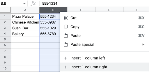
We'll write our CONCATENATE function in this column, so by the end of this tutorial, your combined results will populate in this new column.
2. Write the function in the first cell in your new column.
Select the first cell in your new column and begin typing your function, =CONCATENATE(.

Your strings represent the information that you want to combine. You can select a specific cell to pull the data from that cell, use text in quotation marks ("), or specify a range of cells. In this case, let’s combine A1 with B1 so that the restaurant is in the same cell as its corresponding phone number. Remember to separate your strings with commas:
=CONCATENATE(A1,B1)
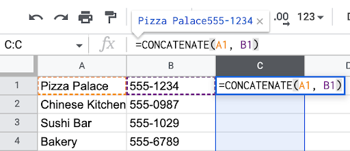
In the example above, you’ll notice that a preview of the results appears above the function. You can use this to ensure you’re concatenating the right strings. Press the enter key to formulate your results in the new column:
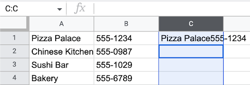
3. Copy and paste the function throughout the column to concatenate other cells.
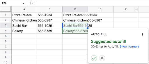
You can replicate the function throughout your column by copying and pasting your function throughout the column, or by clicking on the cell with the function and dragging the bottom right corner.
Google Sheets may also suggest the autofill function, which will automatically populate your column with your function. You can double-check the formula by clicking on the 'Show formula' hyperlink in the autofill suggestion box:
How to concatenate columns in Google Sheets
If you want to concatenate multiple strings, you can replace your comma with a colon to specify a range of cells. For example, =CONCATENATE(A1:B4) will produce the same result as =CONCATENATE(A1, B1, A2, B2, A3, B3, A4, B4). When working with ranges of cells, they are adjoined across rows, then down columns.
Let’s try concatenating two single columns (column A and column B) from the example above:
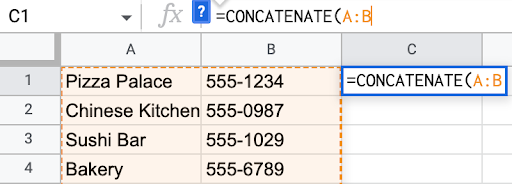
When you begin typing the range, Google Sheets will highlight the cells that you’ve included. Close the parentheses and hit enter to combine the columns into a new cell:

How to add a space when CONCATENATING in Google Sheets
The cells you concatenate are not formatted automatically. This lack of formatting can affect the readability of your data. You can combine cells with spaces in between by including an empty string in your formula. To create an empty string, add a single space enclosed in quotation marks:
=CONCATENATE(A1," ",B1)
You’ll need to include an empty string in between each string that requires a space.
Concatenating dates and times in Google Sheets
If you’re trying to concatenate cells containing dates and times in Google Sheets, you’ll need to take a different approach. There are two ways to join cells with dates and times. The one you’ll use depends on how you formatted your dates.
1. mm/dd/yyyy format
You can join this format using a formula. First, select your cell to the right or left of the ones you’d like to combine. Then, type an equal sign into the function (fx) bar followed by the cells you want to combine. Instead of separating them with a comma, you’ll need to separate them with a plus sign (+), like this: =A1+B1.

A preview of your resulting cell will appear above the formula bar, the same way it would if you were using the concatenate function.
2. mm.dd.yyyy format
Joining cells with this type of date format requires you to use two TEXT functions:
=TEXT(number, format)&TEXT(number, format)
Here, the number is the date or time, and the format is how you want the date or time formatted, written inside quotation marks (").
For example, to combine a date in A1 with a time in A2, you may write:
=TEXT(A1,"mm.dd.yyyy")&TEXT(A2,"hh:mm")
Here,
A1 is your date cell
"mm.dd.yyyy" is your date format
& tells Google Sheets to combine the two text functions
A2 is your time cell
"hh:mm" is your time format

Discover more free resources to help with data analysis
Whether you’re switching or starting a career in data analysis or looking to build your skill set, free resources like Career Chat, our weekly newsletter, can help. Or, you can explore one or more of the following:
Take a quiz: Career Aptitude Quiz
Watch a YouTube video: Is Data Analytics Really That Hard? Tips for Rising to the Challenge
Hear from an expert: 6 Questions with an IBM Data Scientist and AI Engineer
You can also learn and earn credentials at your own pace with Coursera Plus. With a monthly or annual subscription, you can unlock access to more than 10,000 programs from over 350 leading companies and universities.
Coursera Staff
Editorial Team
Coursera’s editorial team is comprised of highly experienced professional editors, writers, and fact...
This content has been made available for informational purposes only. Learners are advised to conduct additional research to ensure that courses and other credentials pursued meet their personal, professional, and financial goals.
